


Next: Master Equation II: the
Up: Master Equation I: Derivation
Previous: Born Approximation
Contents
Index
The equation of motion Eq.(7.20) is pretty useless
unless one specifies at least some more details for the interaction Hamiltonian
 . Denoting system operators by
  and bath operators
by
and bath operators
by  , the most general form of
  is
is
 |
|
|
(23) |
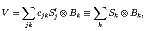
where we have re-defined the sum over  as a new system operator
(
as a new system operator
(
 similarity to Schmid-decomposition).
Remark: Note that  and need not necessarily be hermitian.
Inserting Eq.(7.23) into Eq.(7.22), we have
and need not necessarily be hermitian.
Inserting Eq.(7.23) into Eq.(7.22), we have
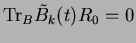
To simplify things, we will assume
 |
|
|
(24) |
from now on. This is no serious restriction.
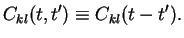
We furthermore introduce the bath correlation functions
![$\displaystyle C_{kl}(t,t')\equiv {\rm Tr}_B \left[\tilde{B}_k(t)\tilde{B}_l(t')R_0\right].$](img103.png) |
|
|
(25) |
Assumption 1:
![$\displaystyle [R_0,H_B]=0$](img104.png) bath in equilibrium bath in equilibrium |
|
|
(26) |
This means
 |
|
|
(27) |
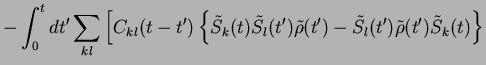
We then have
Assumption 2a (Markov approximation):
the bath correlation function
 is strongly
peaked around
is strongly
peaked around
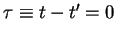 with a peak width
 , where
 is a `typical rate of change of
 .'
Note that
the condition
can only be checked after the equation of motion
for
.'
Note that
the condition
can only be checked after the equation of motion
for
 has been solved.
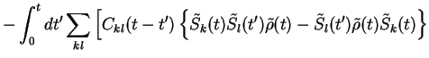
In the interaction picture, one then replaces
has been solved.
In the interaction picture, one then replaces
 under the
integral to obtain
under the
integral to obtain
The important fact is that this approximation is carried out in the interaction (and not in the original
Schrödinger) picture: in the interaction picture, the only relevant time-scale the change of
the density matrix is
 and not (the usually much faster) timescales from the
free evolution with
and not (the usually much faster) timescales from the
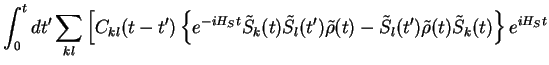
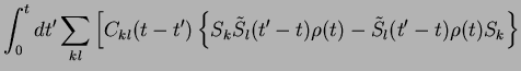
free evolution with  . In fact, one now transforms back into the
Schrödinger picture, using Eq.(7.14),
. In fact, one now transforms back into the
Schrödinger picture, using Eq.(7.14),
which leads to
Assumption 2b (Markov approximation): the integral over  can be carried out to
  .
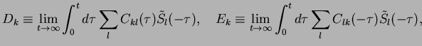
This in fact is completely consistent with assumption 2a (see above). Defining
.
This in fact is completely consistent with assumption 2a (see above). Defining
 |
|
|
(32) |
we can write
![$\displaystyle \fbox{$ \begin{array}{rcl} \displaystyle \frac{d}{dt}\rho(t) &=& ...
... {\rho}(t)
{S}_k+
{\rho}(t)E_k {S}_k - {S}_k{\rho}(t)
E_k \Big].\end{array}$\ }$](img128.png) |
|
|
(33) |
Next: Master Equation II: the
Up: Master Equation I: Derivation
Previous: Born Approximation
Contents
Index
Tobias Brandes
2004-02-18

![$\displaystyle i[H_S,\tilde{\rho}(t)] + e^{iH_S t} \frac{d}{dt}\rho(t) e^{-iH_St}$](img117.png)

![$\displaystyle -i[H_S,{\rho}(t)] + e^{-iH_S t} \frac{d}{dt}\tilde\rho(t) e^{iH_St}$](img119.png)
![$\displaystyle C_{lk}(t'-t)\left\{e^{-iH_S t}
\tilde{\rho}(t)\tilde{S}_l(t') \tilde{S}_k(t) - \tilde{S}_k(t)\tilde{\rho}(t)
\tilde{S}_l(t') \right\}e^{iH_St}\Big]$](img122.png)
![$\displaystyle C_{lk}(t'-t)\left\{
{\rho}(t)\tilde{S}_l(t'-t) {S}_k - {S}_k{\rho}(t)
\tilde{S}_l(t'-t) \right\}\Big].$](img124.png)
![$\displaystyle -i \sum_k{\rm Tr}_B [\tilde{S}_k(t) \tilde{B}_k(t),
R_0 \rho(t=0)]$](img99.png)
![$\displaystyle \int_0^t dt'\sum_{kl}{\rm Tr}_B[\tilde{S}_k(t) \tilde{B}_k(t),
[\tilde{S}_l(t') \tilde{B}_l(t'),R_0 \tilde{\rho}(t')]].$](img101.png)
![$\displaystyle C_{lk}(t'-t)\left\{
\tilde{\rho}(t')\tilde{S}_l(t') \tilde{S}_k(t) - \tilde{S}_k(t)\tilde{\rho}(t')
\tilde{S}_l(t') \right\}\Big].$](img108.png)
![$\displaystyle C_{lk}(t'-t)\left\{
\tilde{\rho}(t)\tilde{S}_l(t') \tilde{S}_k(t) - \tilde{S}_k(t)\tilde{\rho}(t)
\tilde{S}_l(t') \right\}\Big].$](img115.png)