Mapping onto harmonic oscillator master equation

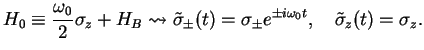
We now use the fact that $H_{SB}$ has the same form as for the the damped single bosonic mode if we identify $\sigma_+\to a^{\dagger}$, $\sigma_-\to a$. We can therefore `copy' the derivation of the master equation of the damped harmonic oscillator, as long as no commutation relations are used! This is the case up to Eq.(7.46),

$$\frac{d}{dt}\rho(t) = -i[\Omega a^{\dagger}a,{\rho}(t)]$$

$$- \frac{1}{2}\Big\{ \left[(\gamma_+ + 2 i \Delta_+)a^{\dagger} a + (\gamma + 2i \Delta) a a^{\dagger}\right]{\rho}(t)$$

$$+ {\rho}(t) \left[ (\gamma - 2i \Delta) a a^{\dagger} + (\gamma_+ -2i \Delta_+) a^{\dagger} a\right]$$

$$- 2\gamma_+ a{\rho}(t)a^{\dagger} -2\gamma a^{\dagger}{\rho}(t)a \Big\}, .$$

The interaction picture for the two-level atom is with respect to the Hamiltonian

$$H_0\equiv \frac{\omega_0}{2}\sigma_z+H_B\leadsto \tilde{\sigma}_{\pm}(t) = \sigma_{\pm} e^{\pm i\omega_0 t},\quad \tilde{\sigma}_{z}(t)=\sigma_z.$$ (125)

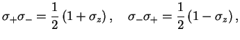
In the interaction picture, the Master equation for the two-level atom therefore reads

$$\frac{d}{dt} \tilde{\rho}(t) = -\frac{1}{2}\Big\{ \left[(\gamma_+ + 2 i \Delta_+) \sigma_+ \sigma_- + (\gamma + 2i \Delta) \sigma_-\sigma_+ \right]\tilde{\rho}(t)$$

$$+ \tilde{\rho}(t) \left[ (\gamma - 2i \Delta) \sigma_-\sigma_+ + (\gamma_+ -2i \Delta_+) \sigma_+ \sigma_- \right]$$

$$- 2\gamma_+ \sigma_-\tilde{\rho}(t)\sigma_+ -2\gamma \sigma_+\tilde{\rho}(t)\sigma_- \Big\}.$$ (126)

We now use

$$\sigma_+\sigma_-=\frac{1}{2}\left(1+\sigma_z\right),\quad \sigma_-\sigma_+=\frac{1}{2}\left(1-\sigma_z\right),$$ (127)

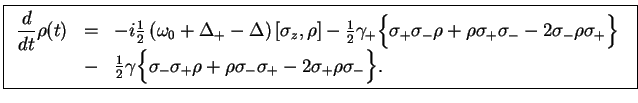
re-arrange and transform back into the Schrödinger picture,

$$\fbox{$ \begin{array}{rcl} \displaystyle \frac{d}{dt}{\rho}(t) &=... ..._+\rho + \rho \sigma_- \sigma_+ -2\sigma_+{\rho}\sigma_-\Big\}. \end{array}$\ }$$ (128)

We recall (note that the harmonic oscillator frequency $\Omega$ has to be replaced by $\omega_0$)

$$\gamma_+ \equiv 2\pi \rho(\omega_0)[1+n_B(\omega_0)],\quad \gamma\equiv 2\pi \rho(\omega_0) n_B(\omega_0)$$

$$\Delta_+ -\Delta \equiv \delta \omega_0 \equiv P\int_{0}^{\infty}d\omega\frac{\rho(\omega)[1+2n_B(\omega)] }{\omega_0-\omega}.$$ (129)

Remarks:

• In contrast to the harmonic oscillator, the energy shift $\hbar \delta\omega_0$ is now temperature dependent.
• The $T=0$ contribution is the Lamb-shift within RWA.