Next: Applications: Linear Coupling, Damped
Up: Influence Functional for Coupling
Previous: Influence Phase
Contents
Index
Linear Response, Fluctuation-Dissipation Theorem for 
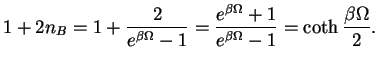
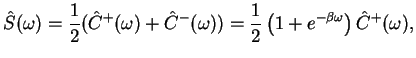
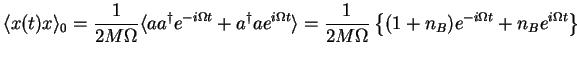
We first check that
 |
|
|
(186) |
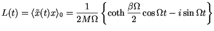
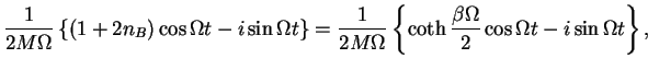
the (van-Hove) position correlation function of the harmonic oscillator with co-ordinate  in thermal
equilibrium: write
in thermal
equilibrium: write
where we again have used the relation
 |
|
|
(188) |
Now let us have another look at this function. Consider the Hamiltonian
![$\displaystyle H_B[x] + H_{SB}[xq]\equiv H(t) = \frac{p^2}{2M}+ \frac{1}{2}M\Omega^2 x^2 + f(t) x,$](img834.png) |
|
|
(189) |
where we consider the function
![$ f[q_t]=f(t)$](img835.png) for a fixed path
for a fixed path  as an external classical force
acting on the oscillator. The density matrix
as an external classical force
acting on the oscillator. The density matrix  of the oscillator in the interaction picture fulfills,
cf Eq.(7.9),
of the oscillator in the interaction picture fulfills,
cf Eq.(7.9),
where
 is assumed to be the thermal equilibrium density matrix.
The expectation value of the position is then
is assumed to be the thermal equilibrium density matrix.
The expectation value of the position is then
We check that
![$\displaystyle \langle [\tilde{x}(t),\tilde{x}(t')] \rangle_0 = \langle [\tilde{x}(t-t'),\tilde{x}(0)] \rangle_0$](img847.png) |
|
|
(191) |
(definition of  !) and define the linear susceptibility
![$\displaystyle \chi_{xx}(t-t') \equiv i \theta(t-t') \langle [\tilde{x}(t-t'),\tilde{x}(0)] \rangle_0 ,$](img849.png) |
|
|
(192) |
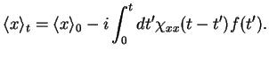
so that we can write
 |
|
|
(193) |
The theta function in
 guarantees causality: the response of at time
  is determined by the system at earlier times
  only.
only.
Define additional functions and their symmetric and antisymmetric (in time) linear combinations,
We thus have
 |
|
|
(195) |
We define the Fourier transforms,
 |
|
|
|
 |
|
|
(196) |
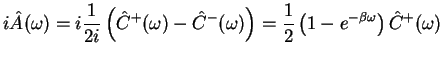
and use
and therefore in the Fourier transform
 (detailed balance relation) (detailed balance relation) |
|
|
(198) |
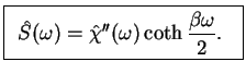
We now define real and imaginary part of the Fourier transform of the susceptibility,
 |
|
|
(199) |
Then,
The relation
 |
|
|
(201) |
is called Fluctuation-Dissipation Theorem (FDT)
(Callen, Welton 1951) and can be re-written, using
 |
|
|
(202) |
leading to
 |
|
|
(203) |
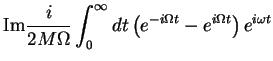
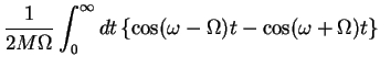
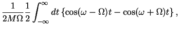
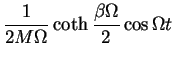
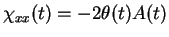
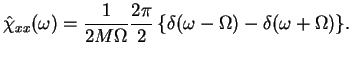
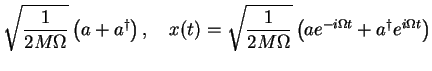
Example- harmonic oscillator: we have
therefore
 |
|
|
(205) |
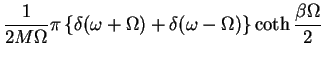
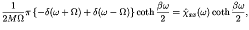
On the other hand,
which is consistent with the FDT.
Next: Applications: Linear Coupling, Damped
Up: Influence Functional for Coupling
Previous: Influence Phase
Contents
Index
Tobias Brandes
2004-02-18
![$\displaystyle {\rho}_0 -i \int_0^t dt'f(t')[\tilde{x}(t'),\tilde{\rho}_B(t')]$](img839.png)
![$\displaystyle {\rho}_0 -i \int_0^t dt'f(t')[\tilde{x}(t'),{\rho}_0]$](img840.png) 1st order
1st order![$\displaystyle \langle x\rangle_0 - i \int_0^t dt' f(t') {\rm Tr} [\tilde{x}(t')...
...\rangle_0 - i \int_0^t dt' f(t') {\rm Tr} {\rho}_0 [\tilde{x}(t),\tilde{x}(t')]$](img845.png)
![$\displaystyle \langle x\rangle_0 - i \int_0^t dt' f(t') \langle [\tilde{x}(t),\tilde{x}(t')] \rangle_0,$](img846.png) 1st order
1st order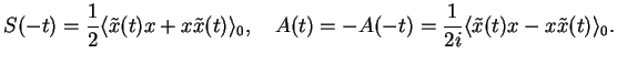

![$\displaystyle i \int_{0}^{\infty} dt \left ( A(t) e^{i\omega t} - \int_{-\infty...
...ga t} \right)
= [A(t)=-A(-t)] = i \int_{-\infty}^{\infty} dt A(t) e^{i\omega t}$](img871.png)
![$\displaystyle i \theta(t) \langle [x(t),x]\rangle_0 = \frac {i \theta(t)}{2M\Omega}
\left(e^{-i\Omega t} - e^{i\Omega t} \right)$](img877.png)