Dipole Approximation

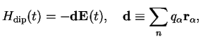
Assume system of charges $q_n$ localised around a spatial position ${\bf r}_0=0$. The coupling to an electric field ${\bf E}({\bf r},t)$ within dipole approximation is then given by

$$H_{\rm dip}(t) = -{\bf d}{\bf E}(t),\quad {\bf d}\equiv \sum_n q_\alpha {\bf r}_\alpha,$$ (2.1)

where ${\bf E}(t)\equiv {\bf E}({\bf r}_0,t)$ is the electric field at ${\bf r}_0=0$. The dipole approximation is valid if the spatial variation of ${\bf E}({\bf r},t)$ around ${\bf r}_0$ is important only on length scales $l$ with $l\gg a$, where $a$ is the size of the volume in which the charges are localised. For a plane wave electric field with wave length $\lambda$ one would have $l \sim \lambda$.