


Next: Breakdown of the Born-Oppenheimer
Up: The Born-Oppenheimer Approximation
Previous: Discussion of the Born-Oppenheimer
Contents
Index
The electronic part equation
usually should give not only one but a whole set of eigenstates,
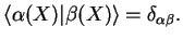
Assume that for a fixed
 we have orthogonal basis of the electronic Hilbert space with states
 , no degeneracies and a discrete spectrum
 ,
,
 |
|
|
(2.14) |
Adiabaticity means that when
is changed slowly from
 , the corresponding state slowly changes
from
, the corresponding state slowly changes
from
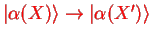 and does not jump to another
 like
like
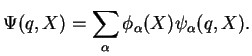
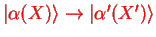 . In that case, we can use the
as a basis for all
and write
. In that case, we can use the
as a basis for all
and write
 |
|
|
(2.15) |
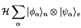
Now
and taking the scalar product with a
 of the Schrödinger equation
 therefore gives
![$\displaystyle \left[\langle \psi_\alpha\vert \mathcal{H}_{\rm n}\vert\psi_\alph...
...pha(X)\right] \vert\phi_\alpha\rangle_n
= \mathcal{E} \vert\phi_\alpha\rangle_n$](img801.png) |
|
|
(2.17) |
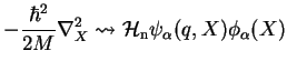
This is the Schrödinger equation for the nuclei within the adiabatic approximation. Now using again
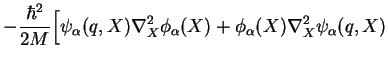
and therefore the nuclear Schrödinger equation becomes
which can be re-written as
where we followed the notation by Mead and Truhlar in their paper J. Chem. Phys. 70, 2284 (1979).
Eq. (E.5.2) is an important result as it shows that the adiabatic assumption leads to extra terms
 and
and
 in the nuclear Schrödinger equation in BO approximation on top of just the potential created by the electrons. In particular, the term
is important as it leads to a non-trivial geometrical phase in cases where the curl of
is non-zero. This has consequences for molecular spectra, too. geometric phases such as the abelian Berry phase and the non-abelian Wilczek-Zee holonomies play an important role in other areas of modern physics, too, one example being `geometrical quantum computing'.
For more info on the geometric phase in molecular systems, cf. the Review by C. A. Mead, Prev. Mod. Phys. 64, 51 (1992).
in the nuclear Schrödinger equation in BO approximation on top of just the potential created by the electrons. In particular, the term
is important as it leads to a non-trivial geometrical phase in cases where the curl of
is non-zero. This has consequences for molecular spectra, too. geometric phases such as the abelian Berry phase and the non-abelian Wilczek-Zee holonomies play an important role in other areas of modern physics, too, one example being `geometrical quantum computing'.
For more info on the geometric phase in molecular systems, cf. the Review by C. A. Mead, Prev. Mod. Phys. 64, 51 (1992).
Next: Breakdown of the Born-Oppenheimer
Up: The Born-Oppenheimer Approximation
Previous: Discussion of the Born-Oppenheimer
Contents
Index
Tobias Brandes
2005-04-26
![$\displaystyle \sum_\alpha \left[ \mathcal{H}_{\rm n} + E_\alpha(X)\right] \vert\phi_\alpha\rangle_n \otimes \vert\psi_\alpha\rangle_e,$](img798.png)
![$\displaystyle 2 \nabla_X \phi_\alpha(X) \nabla_X \psi_\alpha(q,X)\Big]$](img805.png)
![$\displaystyle \left[-\frac{\hbar^2}{2M}\nabla_X^2 +E_\alpha(X) - \langle \psi_\...
...\nabla_X}{M}\vert \psi_\alpha\rangle \nabla_X \right]
\vert\phi_\alpha\rangle_n$](img807.png)
![$\displaystyle \left[-\frac{\hbar^2}{2M}\nabla_X^2 +E_\alpha(X) -\frac{\hbar^2}{2M}G(X) -\frac{\hbar^2}{M}F(X)\nabla_X
\right]
\vert\phi_\alpha\rangle_n$](img809.png)