Correlation Functions

Correlation functions are important since they can tell us a lot about the dynamics of dissipative systems. Moreover, they are often directly related to experimentally accessible quantities, such as photon or electron noise. In quantum optics, fluctuations of the photon field are expressed by correlations functions such as $g^{(1)}(\tau)$ and $g^{(2)}(\tau)$.

We would like to calculate the correlation function of two system operators $A$ and $B$,

$$\fbox{$ \begin{array}{rcl} \displaystyle C_{BA}(t,\tau)&\equiv& \... ...{\rm total} \left( \chi(0) B(t) A(t+\tau) \right),\quad \tau>0. \end{array}$\ }$$ (98)

We insert the time evolution of the operators,

$$\chi(t)=e^{-iHt} \chi(0)e^{iHt},\quad B(t)=e^{iHt} Be^{-iHt},\quad A(t+\tau)=e^{iH(t+\tau)} Ae^{-iH(t+\tau)}$$

to find

$$C_{BA}(t,\tau) = _{\rm total} \left( \chi(0) B(t) A(t+\tau) \right)$$

$$= _{\rm total} \left( e^{iHt}\chi(t) B e^{-iHt}e^{iH(t+\tau)} A e^{-iH(t+\tau)} \right)$$

$$= _{\rm total} \left( e^{-iH\tau}\underline{\chi(t)} B e^{iH\tau} A \right)$$

$$= _{\rm total} \left( e^{-iH\tau}\underline{\rho(t)R_0} B e^{iH\tau} A \right)$$

$$\equiv _{\rm S} \left( A \mbox{\rm Tr}_{\rm Bath} \left\{e^{-iH\tau} \underline{\underline{\rho(t)B}} R_0 e^{iH\tau} \right\}\right)$$

$$\equiv _{\rm S} \left( A \mbox{\rm Tr}_{\rm Bath} \left\{e^{-iH\tau} \underline{\underline{\rho_{B;t}}}R_0 e^{iH\tau} \right\}\right)$$

$$\equiv _{\rm S} \left( A \rho_{B;t}(\tau) \right).$$ (99)

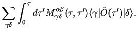
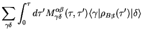
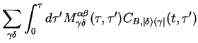
The correlation function can therefore be written as an expectation value of $A$ with a `modified system density matrix' $\rho_{B;t}(\tau)$ which starts at $\tau=0$ as $\rho_{B;t}(\tau=0)=\rho(t)B$ and evolves as a function of time $\tau>0$.

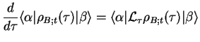
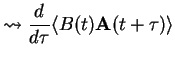
For the time-evolution of a system operator $\hat{O}$ according to

$$\hat{O}(\tau) \equiv _{\rm Bath} \left\{e^{-iH\tau} \hat{O} R_0 e^{iH\tau} \right\},$$ (100)

we can write a formal operator equation

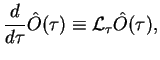$$\frac{d}{d\tau}\hat{O}(\tau) \equiv {\cal L_{\tau}} \hat{O}(\tau),$$ (101)

where we introduced the super-operator ${\cal L_{\tau}}$.

Example: Master equation for $\hat{O} = \rho(0)$ in Born and Markov approximation, cf. Eq.(7.33)

$$\frac{d}{dt}\rho(t) = -i[H_S,{\rho}(t)]$$

$$- \sum_{k}\Big[ {S}_k D_k {\rho}(t) - D_k {\rho}(t) {S}_k+ {\rho}(t)E_k {S}_k - {S}_k{\rho}(t) E_k \Big].$$

It is important to realise that ${\cal L_{\tau}}$ is a linear operator. We now assume that the system has a basis of kets $\{\vert\alpha\rangle \}$ and express the linearity of ${\cal L_{\tau}}$ by writing the matrix elements of ${\cal L_{\tau}} \hat{O}(\tau)$,

$$\langle \alpha \vert {\cal L_{\tau}} \hat{O}(\tau) \vert \beta \rangle = \sum_{\gamma\delta}\int_0^{\tau} d\tau' M^{\alpha\beta}_{\gamma\delta}(\tau,\tau') \langle \gamma \vert \hat{O}(\tau') \vert \delta \rangle.$$ (102)

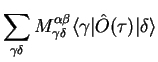
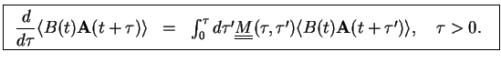
with a time-dependent memory kernel as a fourth-order tensor $M(\tau,\tau')$ that relates the matrix elements of the system operator $\hat{O}$ at earlier times to its matrix elements of the (time-evolved) system operator at later times.

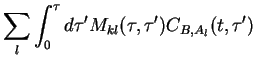
Using now $A=\vert\beta\rangle \langle \alpha\vert$ in $C_{BA}$, we have

$$C_{B,\vert\beta\rangle \langle \alpha\vert}(t,\tau) = \langle \alpha \vert\rho_{B;t}(\tau) \vert \beta\rangle,$$

$$\frac{d}{d\tau}C_{B,\vert\beta\rangle \langle \alpha\vert}(t,\tau) = \frac{d}{d\tau} \langle \alpha \vert\rho_{B;t}(\tau) \vert \beta\rangle= \langle \alpha \vert{\cal L_{\tau}} \rho_{B;t}(\tau) \vert \beta\rangle$$

$$= \sum_{\gamma\delta}\int_0^{\tau} d\tau' M^{\alpha\beta}_{\gamma\delta}(\tau,\tau') \langle \gamma \vert \rho_{B;t}(\tau') \vert \delta \rangle$$

$$= \sum_{\gamma\delta} \int_0^{\tau} d\tau' M^{\alpha\beta}_{\gamma\delta}(\tau,\tau') C_{B,\vert\delta\rangle \langle \gamma\vert}(t,\tau')$$ (103)

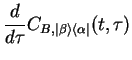
Introducing

$$k \equiv (\alpha \beta),\quad l \equiv (\gamma\delta)$$

$$A_k \equiv \vert\beta\rangle \langle \alpha\vert,\quad M^{\alpha\beta}_{\gamma\delta}(\tau,\tau') \equiv M_{kl}(\tau,\tau'),$$ (104)

we convert the tensor equation into a vector equation,

$$\frac{d}{d\tau}C_{B,A_k}(t,\tau) = \sum_{l} \int_0^{\tau} d\tau' M_{kl}(\tau,\tau') C_{B,A_l}(t,\tau')$$ (105)

which can be written in compact form using the vector of operators,

$${\bf A} \equiv \left(\begin{array}[h]{c} A_1 \\ A_2 \\ .. \\ A_k\\ .. \end{array}\right).$$ (106)

In vector and matrix notation, we thus obtain the quantum regression theorem ,

$$\fbox{$ \begin{array}{rcl} \displaystyle \frac{d}{d\tau}\langle B... ...(\tau,\tau') \langle B(t) {\bf A}(t+\tau')\rangle,\quad \tau>0. \end{array}$\ }$$ (107)

Remarks:

• We have not made use of the Markov approximation here.
• Within the Markov approximation (assumptions 2a and 2b), one has a simple differential (tensor) equation instead of an integro-differential (tensor) equation:
  

  $$\langle \alpha \vert {\cal L_{\tau}} \hat{O}(\tau) \vert \beta \rangle = \sum_{\gamma\delta} M^{\alpha\beta}_{\gamma\delta} \langle \gamma \vert \hat{O}(\tau) \vert \delta \rangle$$

  $$\leadsto \frac{d}{d\tau}\langle B(t) {\bf A}(t+\tau)\rangle = \underline{\underline{M}} \langle B(t) {\bf A}(t+\tau')\rangle,\quad \tau>0.$$ (108)

  
  
  This is the usual form of the quantum regression theorem as discussed in many textbooks.
• For $\tau<0$, the derivation of the quantum regression theorem is analogous to the case $\tau>0$ (exercise!)
• The first derivation of the quantum regression theorem has been given by Melvin Lax, Phys. Rev. 129, 2342 (1963). He emphasises that the only approximation one needs is the factorisation (in our notation $\chi(t)=\rho(t)R_0$, Born approximation). In the `Note added in proof' in his paper he states that the derivation therefore is correct even for non-Markoffian systems.