


Next: Quantum Oscillations in Two-Level
Up: Example: Two-Level System
Previous: Power Series
Contents
Index
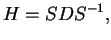
We diagonalise
 according to
 |
|
|
(1.13) |
where
 is the diagonal matrix of the eigenvalues and
 the orthogonal matrix of the eigenvectors.
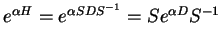
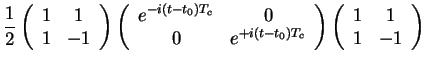
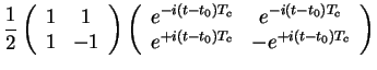
This yields
the orthogonal matrix of the eigenvectors.
This yields
 |
|
|
(1.14) |
which follows from the definition of the power series (Exercise: CHECK)!
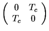
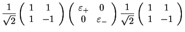
For
 , we already calculated the EVs in an earlier chapter,
with
 . Thus,
Next: Quantum Oscillations in Two-Level
Up: Example: Two-Level System
Previous: Power Series
Contents
Index
Tobias Brandes
2005-04-26
![$\displaystyle \left(\begin{array}{cc}
\cos [(t-t_0)T_c] & -i \sin [(t-t_0)T_c] \\
-i \sin [(t-t_0)T_c] & \cos [(t-t_0)T_c] \\
\end{array}\right)$](img1056.png)