Quantum Oscillations in Two-Level Systems

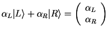
We can now easily calculate these: use an initial condition

$$\vert\Psi\rangle_0 = \alpha_L \vert L\rangle + \alpha_R \vert R\rangle = \left(\begin{array}{c} \alpha_L \alpha_R \end{array}\right)$$

$$\leadsto \vert\Psi(t)\rangle = U(t,t_0) \vert\Psi\rangle_0= \left\{ \cos [(t-t_0)T_c]\hat{1} -i \sin [(t-t_0)T_c] \sigma_x\right\} \vert\Psi\rangle_0$$

$$= \left\{ \alpha_L \cos [(t-t_0)T_c] - i \alpha_R \sin [(t-t_0)T_c] \right\} \vert L\rangle$$

$$+ \left\{ \alpha_R \cos [(t-t_0)T_c] - i \alpha_L \sin [(t-t_0)T_c] \right\} \vert R\rangle.$$ (1.17)

Check out a few examples:

$\alpha_L=1,\alpha_R=0$ (particle initially in left well): in this case, the probabilities for the particle to be in the left (right) well at time $t\ge t_0$ are

$$\vert\langle L \vert\Psi(t)\rangle \vert^2 = \cos ^2[(t-t_0)T_c]$$ (1.18)

$$\vert\langle R \vert\Psi(t)\rangle \vert^2 = \sin ^2[(t-t_0)T_c] .$$