


Next: The Hamiltonian
Up: Gauge invariance for many
Previous: Gauge invariance for many
Contents
Index
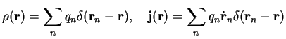
The charge and current density for
 charges
 at positions
 are
are
 |
|
|
(3.1) |
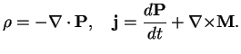
These can be expressed in terms of polarization fields
 (electric polarization) and
 (magnetic polarization or magnetization) via
 |
|
|
(3.2) |
In some traditional formulations of electromagnetism, one distinguishes between `bound' and `free' charges which, however, from a fundamental point of view is a little bit artificial. The above definition of
and
thus refers to the total charge and current charge densities without such separation.
The interesting thing now is the fact that
and
are not uniquely defined by Eq. (VII.3.2). They are arbitrary in very much the same way as the potentials
 and
and
 are arbitrary.
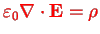
Note that only the longitudinal part of
is uniquely determined from Eq. (VII.3.2) and given by the charge density,
are arbitrary.
Note that only the longitudinal part of
is uniquely determined from Eq. (VII.3.2) and given by the charge density,
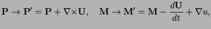
One can transform
and
according to
 |
|
|
(3.4) |
with
 and
and
 still fulfilling Eq. (VII.3.2).
Following Woolley, this arbitraryness is related to charge conservation (I think this interpretation can be carried over to QM and be linked to U(1) invariance of QED). In the classical theory it is the divergence operator playing the central role (
still fulfilling Eq. (VII.3.2).
Following Woolley, this arbitraryness is related to charge conservation (I think this interpretation can be carried over to QM and be linked to U(1) invariance of QED). In the classical theory it is the divergence operator playing the central role (
 , Gauss' law) and the central object in this discussion therefore is the Greens function
 in
in
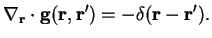 |
|
|
(3.5) |
Fourier transformation yields
In other words, all the arbitraryness (all the fuss about gauge invariance) sits in the transversal part of the
Greens function
of the divergence operator.
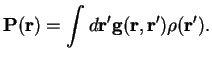
The polarization is now expressed by
that solves
 , i.e.
 |
|
|
(3.7) |
Next: The Hamiltonian
Up: Gauge invariance for many
Previous: Gauge invariance for many
Contents
Index
Tobias Brandes
2005-04-26