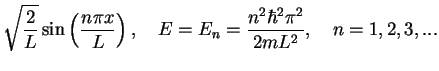
2. The index ![]() is called quantum number, it labels the possible solutions of the
stationary Schrödinger equation
is called quantum number, it labels the possible solutions of the
stationary Schrödinger equation
3. We only have positive integers ![]() : negative integers
: negative integers ![]() would lead to solutions
would lead to solutions
![]() which are just the negative of the wave functions with positive
which are just the negative of the wave functions with positive
![]() . They describe the same state of the particle which is unique up to a phase
. They describe the same state of the particle which is unique up to a phase
![]() (for
example
(for
example
![]() ) anyway.
) anyway.
![]() is linear dependent on
is linear dependent on
![]() .
.
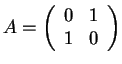
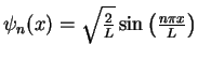
4. The eigenvectors of ![]() , i.e. the functions
, i.e. the functions ![]() , form the basis
of a linear vector space
, form the basis
of a linear vector space ![]() of functions
of functions ![]() defined on the
interval
defined on the
interval ![]() with
with
![]() .
The
.
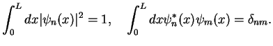
The ![]() form an orthonormal basis:
form an orthonormal basis:
5.
Any wave function
![]() (like any arbitrary vector in, e.g., the vector space
(like any arbitrary vector in, e.g., the vector space ![]() ) can be expanded into
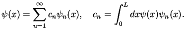
a linear combination of basis `vectors', i.e. eigenfunctions
) can be expanded into
a linear combination of basis `vectors', i.e. eigenfunctions ![]() :
:
| Example | vectors and matrices | Particle in Quantum Well |
| vector | wave function |
|
| space | vector space | Hilbert space |
| linear operator | matrix
 |
Hamiltonian
|
| eigenvalue problem |
|
|
| eigenvalue |
|
|
| eigenvector |
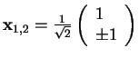 |
wave function
 |
| scalar product |
|
|
| orthogonal basis |
|
|
| dimension | ||
| completeness |
|
|
| vector components |
|
|
We will explain this table in greater detail in the next chapter where we turn to the foundations of quantum mechanics.