Recalling our axioms

In classical mechanics, as described by Newton's equations, a central mathematical object is the phase space, that is the space of all coordinates and momenta $(x_i,p_i)$ of the particles to be described.

Example: A harmonic oscillator of mass $m$ and angular frequency $\omega$ has the energy $H=E=p^2/2m +(1/2)m^2\omega^2 x^2$. For constant energy $E$, its phase space is therefore an ellipse in the $p-x$-plane.

On the other hand, according to Planck, the possible energies of an oscillator are quantized, $E=n\hbar\omega$. In the early days of quantum mechanics, people tried to go on with the concept of the phase space, particle trajectories, and to combine it with quantization rules. However, it became obvious very soon that a more powerful and fundamental theory was needed to explain the spectral lines of atoms. Werner Heisenberg was the one who finally made the breakthrough in 1925 when he stayed a few weeks on the small island of Helgoland in order to cure an attack of hay fever. At that time, he tried to solve a slightly more difficult, non-linear version of the harmonic oscillator. He came up with the idea that instead of trying to find all the trajectories of, for example, electrons in an atom, one should rather consider the entirety of all the frequencies of the spectral lines and their intensities to replace the concept of `trajectories'. This in any case should be more natural since it is the frequencies and intensities which can be observed, not the trajectories of the electrons.

This meant in particular that the concept of the phase space no longer holds in a quantum theory. We already know what one has instead: it is the entity of wave functions that are solutions of the Schrödinger equation. Its stationary solutions at certain energy eigenvalues form the basis of this linear space of wave functions, the Hilbert space ${\cal H}$. We had already discussed an example of a Hilbert space for the solutions of the infinitely high potential well. If you get lost in the following, always have this example in mind:

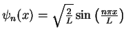
Example: The solutions of the stationary Schrödinger equation for the infinite potential well

$$\psi_n(x) = \sqrt{\frac{2}{L}}\sin \left(\frac{n\pi x}{L}\right ),\quad E= E_n= \frac{n^2 \hbar^2 \pi^2}{2mL^2},\quad n=1,2,3,...$$

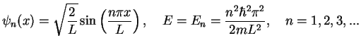
We have learned how to work with wave functions, to calculate probabilities, transmission and reflection coefficients, possible energy values etc. In the following two or three more abstract sections, the wave functions are regarded as vectors, i.e. elements of a vector space.

You certainly know what a vector space is; always have in mind the three-dimensional real vector space $R^3$ where one can add and subtract vectors ${\bf x}$, and multiply vectors with real numbers. The vector spaces of quantum mechanics in general are complex (i.e. you multiply vectors with complex numbers) and, in contrast to $R^3$, often of infinite dimension. But this is not very astonishing to us as we already know by heart our example wave functions $\psi_n$ of the potential well, which form an infinitely dimensional basis.

For convenience, we recall the table we used earlier:

Example	vectors and matrices	Particle in Quantum Well
vector	${\bf x}$	wave function $\psi(x)$
space	vector space	Hilbert space
linear operator	matrix 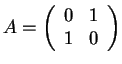$A=\left( \begin{array}{ll} 0&1\\ 1&0 \end{array}\right)$	Hamiltonian $H_{\rm well}$
eigenvalue problem	$A{\bf x} = \lambda {\bf x}$	$H_{\rm well} \psi_n = E_n \psi_n$
eigenvalue	$\lambda_1 = 1,\lambda_2=-1$	$E_n =\frac{n^2\pi^2\hbar^2}{2mL},n=1,2,3...$
eigenvector	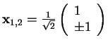${\bf x}_{1,2}=\frac{1}{\sqrt{2}}\left( \begin{array}{l} 1\\ \pm 1 \end{array}\right)$	wave function $\psi_n(x)=\sqrt{\frac{2}{L}}\sin \left(\frac{n\pi x}{L}\right )$
scalar product	$\langle {\bf x} \vert {\bf y} \rangle \equiv \sum_{n=1}^2 x_n^*y_n$	$\langle \psi \vert \phi \rangle \equiv \int_0^Ldx \psi^*(x)\phi(x)$
orthogonal basis	$\langle {\bf e}_n \vert {\bf e}_m \rangle=\delta_{nm}$	$\langle \psi_n \vert \psi_m \rangle =\delta_{nm}$
dimension	$2$	$\infty$
completeness	${\bf x}=\sum_{n=1}^2\langle {\bf e}_n\vert{\bf x} \rangle{\bf e}_n$	$\psi =\sum_{n=1}^{\infty}\langle \psi_n \vert \psi \rangle \psi_n$
vector components	${\bf x} = (\langle {\bf e}_1\vert{\bf x} \rangle,\langle {\bf e}_2\vert{\bf x} \rangle)$	$\psi = (\langle \psi_1 \vert \psi \rangle, \langle \psi_2 \vert \psi \rangle,...)$