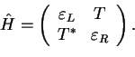
In the previous section we had seen that the total energy of the two tunnel-coupled wells
is represented by the total Hamiltonian ![]() ,
,
If we measure the energy, the possible outcomes are the eigenvalues of the corresponding observable, that
is the total Hamiltonian ![]() . We therefore have to find the two eigenvectors
. We therefore have to find the two eigenvectors
![]() and eigenvalues
and eigenvalues
![]() of
of ![]() , that is the solutions of
, that is the solutions of
Discussion:
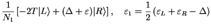
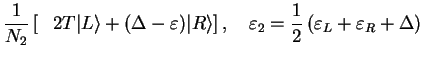
1. The eigenvectors ![]() and
and ![]() form a new orthonormal basis of the Hilbert
space
form a new orthonormal basis of the Hilbert
space
![]() (the
(the ![]() are normalization factors).
are normalization factors).
2. The level splitting ![]() gives the energy difference between the
new eigenenergies. It increases with increasing
gives the energy difference between the
new eigenenergies. It increases with increasing ![]() .
.
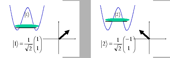
3. For
![]() , we find
, we find
![$\displaystyle \frac{1}{\sqrt{2}}\left[-(T/\vert T\vert) \vert L\rangle + \vert R\rangle \right]$](img896.png)
![$\displaystyle \frac{1}{\sqrt{2}}\left[(T/\vert T\vert) \vert L\rangle + \vert R\rangle \right].$](img897.png)
![$\displaystyle \frac{1}{\sqrt{2}}\left[\vert L\rangle + \vert R\rangle \right],\quad
\varepsilon_1=\varepsilon_0 - \vert T\vert$](img900.png)
![$\displaystyle \frac{1}{\sqrt{2}}\left[ -\vert L\rangle + \vert R\rangle \right],\quad
\varepsilon_2= \varepsilon_0 + \vert T\vert.$](img901.png)