Time Evolution of States

To start with, we simply recall our first axiom of quantum mechanics here:

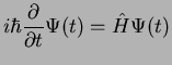
Axiom 1: A quantum mechanical system is described by a vector $\vert\Psi(t)\rangle\equiv \Psi(t)$ of a Hilbert space ${\cal H}$. The time evolution of $\Psi(t)$ is determined by the Schrödinger equation

$$i\hbar\frac{\partial}{\partial t} \Psi(t) = \hat{H} \Psi(t)$$ (211)

The Hamilton operator $\hat{H}$ is an operator corresponding to the total energy of the system. The solutions of the stationary Schrödinger equation at fixed energy,

$$\hat{H}\phi=E\phi$$ (212)

are called stationary states, the possible energies $E$ eigenenergies.

We now specialize everything to our two-level system:

Hilbert space	${\cal H} = C^2$	2d complex vector space
Basis vectors	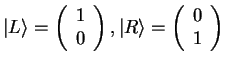$\vert L\rangle = \left(\begin{array}{c} 1 \\ 0 \end{array}\right), \vert R\rangle= \left(\begin{array}{c} 0 \\ 1 \end{array}\right)$	particle left or right
Arbitrary vector	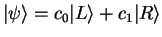$\vert\psi\rangle = c_0 \vert L\rangle + c_1 \vert R\rangle$, $\vert c_0\vert^2+\vert c_1\vert^2=1$	particle in arbitrary state
Hamiltonian	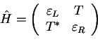$$\hat{H}=\left( \begin{array}{cc} \varepsilon_L & T\\ T^* & \varepsilon_R \end{array}\right)$$	two-dimensional matrix
Stationary states	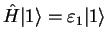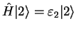$\hat{H}\vert 1\rangle = \varepsilon_1 \vert 1\rangle$, $\hat{H}\vert 2\rangle = \varepsilon_2 \vert 2\rangle$	The two energy eigenstates

Time evolution means the following: Suppose the state of the quantum system at time $t=0$ is $\vert\Psi(t=0)\rangle =\vert\Psi_0\rangle$. Then, the solution of the time-dependent Schrödinger equation $i\hbar\partial_t \Psi(t) = \hat{H} \Psi(t)$ gives us the state $\vert\Psi(t)\rangle$ at a later time $t>0$.

CASE 1: Time evolution of a stationary state

If the initial state $\vert\Psi_0\rangle$ is a stationary state, the time-evolution is simple:

$$\vert\Psi(t=0)\rangle = \vert 1\rangle \leadsto \vert\Psi(t>0)\rangle = \vert 1\rangle e^{-i\varepsilon_1 t/\hbar}$$

$$\vert\Psi(t=0)\rangle = \vert 2\rangle \leadsto \vert\Psi(t>0)\rangle = \vert 2\rangle e^{-i\varepsilon_2 t/\hbar}$$ (213)

because

$$i\hbar \frac{\partial}{\partial t}\vert\Psi(t)\rangle = i\hbar \frac{\partial}{\partial t} \vert 1\rangle e^{-i\varepsilon_1 t/\hbar} = \underline{\varepsilon_1 \vert 1\rangle} e^{-i\varepsilon_1 t/\hb... ...hat{H} \vert 1\rangle} e^{-i\varepsilon_1 t/\hbar}=\hat{H} \vert\Psi(t)\rangle.$$ (214)

(the same for $\vert\Psi(t=0)\rangle = \vert 2\rangle$). The time-evolution is `trivial' and just given by the phase factor $e^{-iEt/\hbar}$, where $E$ is the eigenenergy of the stationary state.

CASE 2: Time evolution of a superposition of the two energy eigenstates

$$\vert\Psi(t=0)\rangle = \alpha_1 \vert 1\rangle + \alpha_2 \vert 2\rangle \leadsto \vert\... ...{-i\varepsilon_1 t/\hbar} + \alpha_2 \vert 2\rangle e^{-i\varepsilon_2 t/\hbar}$$ (215)

because

$$i\hbar \frac{\partial}{\partial t}\vert\Psi(t)\rangle = i\hbar \frac{\partial}{\partial t}\left[\alpha_1 \vert 1\rangle e... ...repsilon_1 t/\hbar} +\alpha_2 \vert 2\rangle e^{-i\varepsilon_2 t/\hbar}\right]$$

$$= \alpha_1{\varepsilon_1 \vert 1\rangle} e^{-i\varepsilon_1 t/\hbar} +\alpha_2{\varepsilon_2 \vert 2\rangle} e^{-i\varepsilon_2 t/\hbar}$$

$$= \hat{H} \alpha_1 \vert 1\rangle e^{-i\varepsilon_1 t/\hbar} +\hat... ...lpha_2 \vert 2\rangle e^{-i\varepsilon_2 t/\hbar} =\hat{H} \vert\Psi(t)\rangle.$$ (216)

To obtain the time evolution of an arbitrary initial state $\vert\Psi(t=0)\rangle$, we therefore have to do the following: decompose $\vert\Psi(t=0)\rangle$ into a linear combination of energy eigenstates ($\vert 1\rangle$ and $\vert 2\rangle$). Then, simply dress the stationary states in this linear combination with the phase factors $e^{-i\varepsilon_1t/\hbar}$ and $e^{-i\varepsilon_2t/\hbar}$. The linearity of the Schrödinger equation makes it that simple: the time evolution of a sum of stationary states is the sum of the time-evolved linear components of this sum.

The calculational effort is in the determination of the coefficients $\alpha_1$ and $\alpha_2$: we discuss this in the special

CASE 3: The initial state is $\vert\Psi(t=0)\rangle = \vert L\rangle$, describing the particle in the left well. Note that we don't have simply a time evolution given by a phase factor:

$$\vert\Psi(t=0)\rangle = \vert L\rangle \leadsto \vert\Psi(t>0)\rangle {\bf\ne} e^{-iEt/\hbar} \vert L\rangle \mbox{\rm for some $E$} .$$

The state $\vert L\rangle$ is not an eigenstate of the Hamiltonian $\hat{H}$, therefore its time evolution is not given by a simple phase factor. What we have to do is clear: we have to find the decomposition of the vector $\vert L\rangle$ into a linear combination of energy eigenstates $\vert 1\rangle$ and $\vert 2\rangle$,

$$\vert\Psi(t=0)\rangle = \vert L\rangle = \alpha_1 \vert 1\rangle ... ...-i\varepsilon_1 t/\hbar} + \alpha_2 \vert 2\rangle e^{-i\varepsilon_2 t/\hbar}.$$ (217)

For simplicity, we do this for the special case of negative $T$ and identical energy parameters $\varepsilon_L=\varepsilon_R$ in the Hamiltonian $\hat{H}$. We had calculated already before in (3.41),

$$\varepsilon_L=\varepsilon_R=:\varepsilon_0,\quad T=-\vert T\vert\leadsto \vert 1\rangle = \frac{1}{\sqrt{2}}\left[\vert L\rangle + \vert R\rangle \right],\quad \varepsilon_1=\varepsilon_0 - \vert T\vert$$

$$\vert 2\rangle = \frac{1}{\sqrt{2}}\left[ -\vert L\rangle + \vert R\rangle \right],\quad \varepsilon_2= \varepsilon_0 + \vert T\vert.$$ (218)

We solve this equation for $\vert L\rangle$,

$$\vert L\rangle = \frac{1}{\sqrt{2}}\left[ \vert 1\rangle - \vert 2\rangle \right]\leadsto \alpha_1 = \frac{1}{\sqrt{2}},\quad \alpha_2 = -\frac{1}{\sqrt{2}}.$$ (219)

By this we have found our desired result, that is the time evolution of the initial state $\vert L\rangle$,

$$\vert\Psi(t=0)\rangle = \vert L\rangle \leadsto \vert\Psi(t)\rangle = \frac{1}{\sqrt{2}}\left[ \vert 1\rangle e^{-i\varepsilon_1 t/\hbar} - \vert 2\rangle e^{-i\varepsilon_2 t/\hbar}\right].$$ (220)

We have expressed $\vert\Psi(t)\rangle$ in the basis of the energy eigenstates $\vert 1\rangle$ and $\vert 2\rangle$. We now would like to express $\vert\Psi(t)\rangle$ in the basis of the left and right states, $\vert L\rangle$ and $\vert R\rangle$: this is simple because we know

$$\vert 1\rangle = \frac{1}{\sqrt{2}}\left[\vert L\rangle + \vert R\rangle \right],\... ...rt 2\rangle = \frac{1}{\sqrt{2}}\left[ -\vert L\rangle + \vert R\rangle \right]$$

$$\leadsto \underline{\vert\Psi(t)\rangle} = \frac{1}{\sqrt{2}}\left[ \vert 1\rangle e^{-i\varepsilon_1 t/\hbar} - \vert 2\rangle e^{-i\varepsilon_2 t/\hbar}\right] =$$

$$= \frac{1}{{2}}\left\{ \left[\vert L\rangle + \vert R\rangle \right... ...[-\vert L\rangle + \vert R\rangle \right] e^{-i\varepsilon_2 t/\hbar}\right\} =$$

$$= \frac{1}{{2}}\left\{\vert L\rangle \left[e^{-i\varepsilon_1 t/\hb... ... \left[e^{-i\varepsilon_1 t/\hbar} - e^{-i\varepsilon_2 t/\hbar}\right]\right\}$$

$$=: \underline{c_0(t)\vert L\rangle + c_1(t)\vert R\rangle}$$

$$c_0(t) := \frac{1}{{2}}\left[e^{-i\varepsilon_1 t/\hbar} + e^{-i\varepsilon... ...{1}{{2}}\left[e^{-i\varepsilon_1 t/\hbar} - e^{-i\varepsilon_2 t/\hbar}\right].$$ (221)

The coefficients $c_0(t)$ and $c_1(t)$ have a clear physical meaning: let us recall

$$\vert c_0\vert^2(t)=p_0(t) =$$ the probability to find the particle in the left well

$$\vert c_1\vert^2(t)=p_1(t) = .$$ (222)

Obviously, these probabilities are a function of time now: $\vert\Psi(t)\rangle$ is not stationary. We calculate

$$p_0(t) = \frac{1}{{4}}\left\vert e^{-i\varepsilon_1 t/\hbar} + e^{-i\varep... ...2 =\frac{1}{2}\left\{ 1 + \cos [(\varepsilon_1-\varepsilon_2)t/\hbar)] \right\}$$

$$= \cos^2 [\frac{(\varepsilon_1-\varepsilon_2)t}{2\hbar}]$$

$$p_1(t) = \frac{1}{{4}}\left\vert e^{-i\varepsilon_1 t/\hbar} - e^{-i\varep... ...2 =\frac{1}{2}\left\{ 1 - \cos [(\varepsilon_1-\varepsilon_2)t/\hbar)] \right\}$$

$$= \sin^2 [\frac{(\varepsilon_1-\varepsilon_2)t}{2\hbar}]$$ (223)

and therefore

$$\cos^2 [\frac{(\varepsilon_1-\varepsilon_2)t}{2\hbar}] =$$ the probability to find the particle in the left well

$$\sin^2 [\frac{(\varepsilon_1-\varepsilon_2)t}{2\hbar}] = .$$ (224)

As a function of time, the probabilities oscillate with an angular frequency that is given by the energy splitting $\Delta=\varepsilon_2-\varepsilon_1=2\vert T\vert$, divided by $\hbar$. At the initial time $t=0$, the particle is in the left well (the probability $p_0(0)=1$), but for $t>0$ this probability starts to oscillate: the particle tunnels from the left well into the right well, back into the left well and so forth.