Derivation of the PDE

In order to transform the master equation, we require the $P$-representation of terms like $a\rho a^{\dagger}$ etc. Let us start with $a^{\dagger}\rho$.

Method 1: We follow Walls/Milburn and introduce Bargmann states

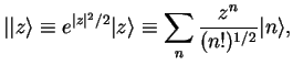$$\vert\vert z\rangle \equiv e^{\vert z\vert^2/2}\vert z\rangle \equiv \sum_n \frac{z^n}{(n!)^{1/2}}\vert n\rangle,$$ (72)

(`coherent states without the normalisation factor in front'). Therefore,

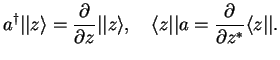$$a^{\dagger}\vert\vert z\rangle = \frac{\partial}{\partial z}\vert... ...ad \langle z \vert\vert a = \frac{\partial}{\partial z^*} \langle z \vert\vert.$$ (73)

We use this to write

$$\rho = \int \frac{d^2 z}{\pi}\vert\vert z\rangle \langle z\vert\vert e^{-\vert z\vert^2} \underline{P(z)} \leadsto$$ (74)

$$a^{\dagger}\rho = \int \frac{d^2 z}{\pi}a^{\dagger} \vert\vert z\rangle \langle z\v... ...tial z} \vert\vert z\rangle \right] \langle z\vert\vert e^{-\vert z\vert^2}P(z)$$

$$= -\int \frac{d^2 z}{\pi} \vert\vert z\rangle \langle z\vert\vert\f... ...vert z\vert^2} \underline{\left( z^*- \frac{\partial}{\partial z}\right) P(z)},$$

using integration by parts, $\frac{\partial}{\partial z}\langle z\vert\vert=0$, and assuming the vanishing of $P(z)$ at infinity. Comparison yields

$$a^{\dagger}\rho \leftrightarrow \left( z^*- \frac{\partial}{\partial z}\right) P(z).$$ (75)

Method 2: Use the Metha formula for $\hat{\theta} = a^{\dagger}\rho$,

$$P(a^{\dagger}\rho;z) = e^{\vert z\vert^2} \int \frac{d^2z'}{\pi} \langle -z'\vert a^{\dagger}\rho \vert z'\rangle e^{\vert z'\vert^2} e^{zz'^*-z^*z'}$$

$$= e^{zz^*} \int \frac{d^2z'}{\pi}(-z'^*) \langle -z'\vert \rho \vert z'\rangle e^{\vert z'\vert^2} e^{zz'^*-z^*z'}=$$

$$= \left[ -\frac{\partial}{\partial z} + z^*\right] (e^{zz^*}) \int ... ...\pi} \langle -z'\vert \rho \vert z'\rangle e^{\vert z'\vert^2} e^{zz'^*-z^*z'}.$$ (76)

Here, we generate $-z'^*$ in the integral by differentiation with respect to the parameter $z$ and subsequent compensation of the term aring from $e^{zz^*}$, thus arriving even faster at Eq.(7.76). Similarly,

$$P(\rho a;z) = e^{zz^*} \int \frac{d^2z'}{\pi} \langle -z'\vert \rho \vert z'\rangle z' e^{\vert z'\vert^2} e^{zz'^*-z^*z'}=$$

$$= \left[ -\frac{\partial}{\partial z^*} + z\right] (e^{zz^*}) \int ... ...\pi} \langle -z'\vert \rho \vert z'\rangle e^{\vert z'\vert^2} e^{zz'^*-z^*z'}.$$ (77)

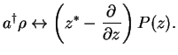
For the terms $a^{\dagger}a\rho$, the first method is easier:

$$a^{\dagger}a\rho = \int \frac{d^2 z}{\pi}a^{\dagger} a \vert\vert z\rangle \langle z... ...l z} \vert\vert z\rangle \right] \langle z\vert\vert e^{-\vert z\vert^2} z P(z)$$

$$= -\int \frac{d^2 z}{\pi} \vert\vert z\rangle \langle z\vert\vert\f... ...ert z\vert^2} \underline{\left( z^*- \frac{\partial}{\partial z}\right) z P(z)}$$

$$\rho a^{\dagger}a = \int \frac{d^2 z}{\pi}\vert\vert z\rangle \langle z\vert\vert a^{... ...c{\partial}{\partial z^*}\langle z\vert\vert\right] e^{-\vert z\vert^2} z^*P(z)$$

$$= -\int \frac{d^2 z}{\pi} \vert\vert z\rangle \langle z\vert\vert\f... ...t z\vert^2} \underline{\left( z- \frac{\partial}{\partial z^*}\right) z^* P(z)}$$

$$a \rho a^{\dagger} = \int \frac{d^2 z}{\pi}a \vert\vert z\rangle \langle z\vert\vert a... ...ert\vert z\rangle \langle z\vert\vert e^{-\vert z\vert^2} \underline{zz^* P(z)}$$

$$a^{\dagger} \rho a = \int \frac{d^2 z}{\pi} \left[\frac{\partial}{\partial z} \vert\ve... ...frac{\partial}{\partial z^*}\frac{\partial}{\partial z}e^{-\vert z\vert^2} P(z)$$

$$= \int \frac{d^2 z}{\pi}\vert\vert z\rangle \langle z\vert\vert e^{... ...tial}{\partial z^*}\right) \left( z^*- \frac{\partial}{\partial z}\right)P(z)}.$$

In particular, for the master equation we need

$$\Big\{ a^{\dagger} a {\rho} + \rho a^{\dagger} a - 2 a \rho a^{\dagger} \Big\} \leftrightarrow \Big\{ \left( z^*- \frac{\partial}{\partial z}\right) z + \left( z- \frac{\partial}{\partial z^*}\right) z^* - 2 zz^* \Big\} P(z)$$

$$= - \Big\{ \frac{\partial}{\partial z} z+\frac{\partial}{\partial z^*} z^*\Big\} P(z) = - \Big\{ z\frac{\partial}{\partial z} +z^*\frac{\partial}{\partial z^*} +2 \Big\} P(z)$$

$$\Big\{ a^{\dagger} a {\rho} +\rho (a^{\dagger}a+1) - a \rho a^{\dagger} -a^{\dagger} \rho a \Big\} \leftrightarrow \Big\{\left( z^*- \frac{\partial}{\partial z}\right) z + \left( z- \frac{\partial}{\partial z^*}\right) z^* +1$$

$$- zz^* - \left( z- \frac{\partial}{\partial z^*}\right) \left( z^*- \frac{\partial}{\partial z}\right)\Big\} P(z)$$

$$=\Big\{-\frac{\partial}{\partial z} z + z \frac{\partial}{\partial z}+1 + \frac{\partial}{\partial z^*} \frac{\partial}{\partial z}\Big\} P(z) = \frac{\partial}{\partial z^*} \frac{\partial}{\partial z}P(z)$$

$$\left[ a^{\dagger} a,\rho \right] \leftrightarrow \left[-\frac{\partial}{\partial z}z + \frac{\partial}{\partial z^... ...ft[-z\frac{\partial}{\partial z} + z^*\frac{\partial}{\partial z^*}\right]P(z).$$

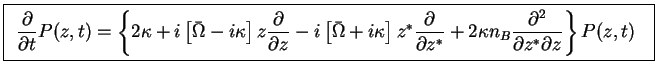
The whole master equation is therefore transformed into

$$\fbox{$ \begin{array}{rcl} \displaystyle \frac{\partial}{\partial... ...n_B \frac{\partial^2}{\partial z^*\partial z}\right\} P(z,t)\\ \end{array}$\ }$$ (78)

Here, we have explicitely indicated that the $P$-function depends both on $z$ and on the time $t$.

Remarks:

• The first order derivate terms are called drift terms, the second order derivate terms diffusion term.
• This is not directly solvable by Fourier transformation: $z$,$z^*$-dependence of coefficients.
• Written in real coordinates, this has the form of a Fokker-Planck equation
  

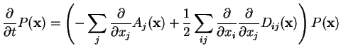  $$\frac{\partial}{\partial t}P({\bf x})=\left( -\sum_j \frac{\parti... ...l}{\partial x_i} \frac{\partial}{\partial x_j}D_{ij}({\bf x}) \right)P({\bf x})$$ (79)