Dipole Approximation

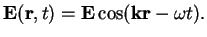
Consider an electrical field in the form of a linearly polarised, monochromatic plain wave with wave vector ${\bf k}$,

$${\bf E}({\bf r},t) = {\bf E} \cos({\bf kr}-\omega t).$$ (114)

Describe the interaction of the atom with the electrical field in dipole approximation: the energy of a dipole ${\bf d}$ in a field ${\bf E}({\bf r},t)$ is given by $-{\bf d E}({\bf r},t)$. Treating the field classically, we obtain the time-dependent dipole Hamiltonian

$$H_L(t) = -\langle g\vert {\bf d E}({\bf r},t)\vert e\rangle \vert g\rangle... ...langle e\vert {\bf d E}({\bf r},t)\vert g\rangle \vert e\rangle \langle g \vert$$

$$\approx - \left(\hbar \Omega \sigma_- + \hbar \Omega^* \sigma_+ \right)\cos(\omega t),$$ (115)

where we used ${\bf kr}\ll 1$ in the overlap integral (wave length $\gg$ dimension of atom, `dipole approximation'), and introduced

$$\sigma_- \equiv \vert g\rangle \langle e\vert,\quad \sigma_+ \equiv \vert e\rangle \langle g\vert.$$ (116)

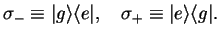
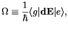
and the Rabi frequency

$$\Omega\equiv \frac{1}{\hbar}\langle g\vert {\bf d E}\vert e\rangle,$$ (117)

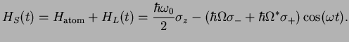
which in general is a complex number. The total system Hamiltonian therefore is

$$H_S(t) = H_{\rm atom}+H_L(t)= \frac{\hbar\omega_0}{2}\sigma_z - \left(\hbar \Omega \sigma_- + \hbar \Omega^* \sigma_+ \right)\cos(\omega t).$$ (118)

One usually assumes real $\Omega=\Omega^*$, in this case we can formally write $H_S(t)={\bf B}(t){\vec{\sigma}}$ with

$${\bf B}(t)=\left( \begin{array}[h]{c} -\hbar\Omega\cos(\omega t)\\ 0\\ \frac{1}{2}\hbar\omega_0 \end{array} \right).$$ (119)