The continuity equation

We generate one equation by multiplying the Schrödinger equation with $\Psi^*(x,t)$, where $^*$ means conjugate complex. We generate another equation by multiplying the (Schrödinger equation)$^*$ with $-\Psi(x,t)$ and add both equations. The result is

$$i\hbar(\Psi^*\partial_t\Psi+\Psi\partial_t\Psi^*) = -\frac{\hbar^2}{2m}\left[ \Psi^*\partial_x^2\Psi- \Psi\partial_x^2\Psi^*\right]$$

$$i\hbar\partial_t(\Psi\Psi^*) = -\frac{\hbar^2}{2m}\partial_x \left[ \Psi^*\partial_x\Psi- \Psi\partial_x\Psi^*\right].$$ (38)

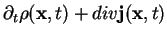
This can be written in the form of a continuity equation:

$$\fbox{$ \begin{array}{rcl} \displaystyle & &\frac{\partial}{\part... ...si(x,t) - \Psi(x,t)\frac{\partial}{\partial x}\Psi^*(x,t)\right]. \end{array}$}$$ (39)

You should check that beside the probability density $\rho(x,t)$ also the probability current density $j(x,t)$ both are real quantities. Eq. (1.39) in fact is the one-dimensional version of a continuity equation

$$\partial_t\rho({\bf x},t)+ div {\bf j}({\bf x},t) =$$ 0 (40)

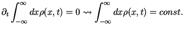
that appears in different areas of physics such as fluid dynamics or wave theory. We note that for simplicity up to here we have only dealt with the one-dimensional version of the Schrödinger equation which yields the one-dimensional version of the continuity equation. We integrate Eq. (1.39) from $x=-\infty$ to $x=\infty$ and assume that $\Psi$ vanishes at infinity which is plausible: if $\Psi$ is related to a probability, this probability should be zero at points of space that are inaccessible to the particles, i.e. at infinity. We obtain

$$\partial_t\int_{-\infty}^{\infty}dx \rho({x},t)=0 \leadsto \int_{-\infty}^{\infty}dx \rho({x},t)= const.$$ (41)

The statistical interpretation of $\Psi(x,t)$ is one of the central axioms of quantum mechanics.