Stationary states

The Schrödinger equation is a partial differential equation: we have one partial derivative with respect of time $t$ and the Laplace operator $\Delta$ which is a differential operator, 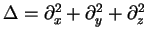$\Delta=\partial_x^2+\partial_y^2+\partial_z^2$ in three dimensions and rectangular coordinates.

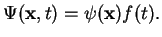
Step 1: To solve (2.1), we make the separation ansatz

$$\Psi({\bf x},t) = \psi({\bf x})f(t).$$ (79)

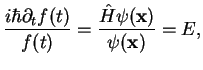
Inserting into (2.1) we have

$$\frac{i\hbar\partial_t f(t)}{f(t)}=\frac{\hat{H}\psi({\bf x})}{\psi({\bf x})}=E,$$ (80)

where we have separated the $t$- and the ${\bf x}$-dependence. Both sides of (2.3) depend on $t$ resp. ${\bf x}$ independently and therefore must be constant $=E$. Solving the equation for $f(t)$ yields $f(t)= \exp[{-iEt/\hbar}]$ and therefore

$$\Psi({\bf x},t) = \psi({\bf x})e^{-iEt/\hbar}.$$ (81)

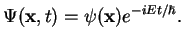
We recognize: the time evolution of the wave function $\Psi({\bf x},t)$ is solely determined by the factor $\exp[{-iEt/\hbar}]$. Furthermore, the constant $E$ must be an energy (dimension!).

Step 2: To determine $\psi({\bf x})$, we have to solve the stationary Schrödinger equation

$${\hat{H}\psi({\bf x}) = E \psi({\bf x})} \longleftrightarrow \left[-\frac{\hbar^2\Delta}{2m} + V({\bf x}) \right]\psi({\bf x})=E\psi({\bf x}).$$ (82)

Mathematically, the equation $\hat{H}\psi=E\psi$ with the operator $\hat{H}$ is an eigenvalue equation. We know eigenvalue equations from linear algebra where $\hat{H}$ is a matrix and $\psi$ is a vector. The time-independent wave functions $\psi({\bf x})$ are called stationary wave functions or stationary states. We will see in the following that in general, solutions of the stationary Schrödinger equation do not exist for arbitrary $E$. Rather, many potentials $V({\bf x})$ give rise to solutions only for certain discrete values of $E$, the eigenvalues of the stationary Schrödinger equation, and the possible energy values become quantized.