


Next: The Tunnel Effect and
Up: Scattering states in one
Previous: Plane waves
Contents
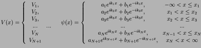
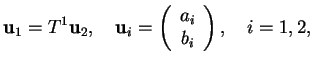
We now consider a piecewise constant potential  with the corresponding wave function given by
 |
(119) |
 .
.
We first consider the case
 such that
  and
and  are real wave vectors
and
are real wave vectors
and  describes running waves outside the `scattering region'
 ![$ [x_1,x_N]$](img521.png) .
Our aim now is the following: we would like to determine solutions of the Schrödinger equation,
i.e. wave functions , under the scattering condition
.
Our aim now is the following: we would like to determine solutions of the Schrödinger equation,
i.e. wave functions , under the scattering condition  , i.e.
we seek solutions that have only waves
, i.e.
we seek solutions that have only waves
 traveling to the right (away from the scattering
zone) on the right side of the potential. On the left side, we have the wave
traveling to the right (away from the scattering
zone) on the right side of the potential. On the left side, we have the wave
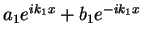 , i.e. a superposition of a right-going (incoming) and a left-going
(outgoing) wave. We would like to know how much of an incoming wave gets reflected
on the left side (coefficient
, i.e. a superposition of a right-going (incoming) and a left-going
(outgoing) wave. We would like to know how much of an incoming wave gets reflected
on the left side (coefficient  ) and how much gets transmitted on the right side (
 ).
).
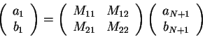
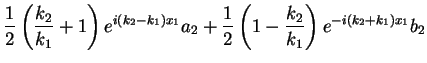
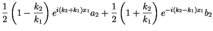
Step 1: we demand that and its derivative  are continuous
at
are continuous
at  . This gives two equations
or
which can be written in a matrix form
 |
(122) |
with
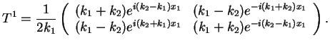 |
(123) |
Step 2: In completely the same manner, we obtain the transfer matrix  at the `slice'
  and
and
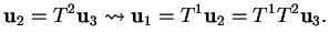 |
(124) |
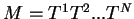
Doing this for all the slices
 , we obtain the complete transfer matrix
  that connects the wave function on the left side of the potential with the one on the right side,
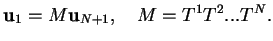 |
(125) |
Step 3:
We use the continuity equation
The current density is time-independent and can be written as
The current density on the right and left side of the potential is
The current density  describes a particle flow to the right of the potential, `out-flowing'
to
describes a particle flow to the right of the potential, `out-flowing'
to
 . On the other hand,
the current density
. On the other hand,
the current density  is the difference of an in-flowing positive current density
and an out-flowing negative current density. The former describes an incoming particle, the latter a
particle that is reflected back from the potential and returning back to
is the difference of an in-flowing positive current density
and an out-flowing negative current density. The former describes an incoming particle, the latter a
particle that is reflected back from the potential and returning back to  .
.
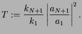
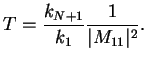
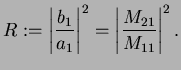
Step 4: We define the transmission coefficient  as the
ratio of the right out-flowing current density to the left in-flowing current density,
as the
ratio of the right out-flowing current density to the left in-flowing current density,
 |
|
|
(130) |
From
 |
|
|
(131) |
and the scattering condition it follows
 |
|
|
(132) |
To calculate the transmission coefficient through a piecewise constant one-dimensional potential,
it is therefore sufficient to know the total transfer matrix . The fact that
 is just the
product of the individual two-by two transfer matrices makes it a very convenient tool for computations.
is just the
product of the individual two-by two transfer matrices makes it a very convenient tool for computations.
Figure:
Reflection and Transmission
|
|
Step 5: In completely the same manner, we define the reflection coefficient  as the
ratio of the out-flowing current density on the left and the in-flowing (reflected) current density on the
left, i.e.
as the
ratio of the out-flowing current density on the left and the in-flowing (reflected) current density on the
left, i.e.
 |
|
|
(133) |
The last equality is left as an exercise.
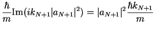
For eigenstates of energy  we have from the continuity equation
 |
|
|
(134) |
Using Eq. (2.52) and the definition of and , this leads to
 |
|
|
(135) |
Next: The Tunnel Effect and
Up: Scattering states in one
Previous: Plane waves
Contents
Tobias Brandes
2004-02-04
![$\displaystyle -\frac{i\hbar}{2m} \left[ \psi(x,t)^*\partial_x\psi(x,t)-
\psi(x,t)\partial_x\psi^*(x,t)\right]$](img548.png)
![$\displaystyle -\frac{i\hbar}{2m} \left[ \psi(x)^*\partial_x\psi(x)-
\psi(x)\partial_x\psi^*(x)\right]= \frac{\hbar}{m}{\rm Im} \left[ \psi^*(x)\psi'(x)\right].$](img552.png)
![$\displaystyle \frac{\hbar}{m}{\rm Im} \left[(a_1^*e^{-ik_1x}+b_1^*e^{ik_1x})ik_1
(a_1e^{ik_1x}-b_1e^{-ik_1x})\right]$](img556.png)
![$\displaystyle \frac{\hbar k_1}{m}[\vert a_1\vert^2 - \vert b_1\vert^2].$](img557.png)
![\includegraphics[width=0.5\textwidth]{qm2_4_1.eps}](img564.png)