Next: The Harmonic Oscillator II
Up: The Harmonic Oscillator I
Previous: Model
Contents
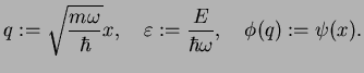
Now we actually want to solve (4.5). We introduce dimensionless quantities
 |
|
|
(230) |
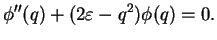
Then, (4.5) becomes
 |
|
|
(231) |
For large
 , one can neglect the term
 . This yields the asymptotic behaviour of
 ,
,
 |
|
|
(232) |
which you can check by differentiating
 |
|
|
(233) |
This roughly is an example of how an asymptotic analysis of a differential equation
is performed; if you are interested for more mathematical details of the interesting
theory of asymptotic analysis have a look at the book by Bender and Orszag.
We obviously have two different solutions: one grows to infinity as
 , while the
other goes to zero. Wave functions have to be normalized which is impossible for the solution
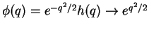
that grows to infinity. We exclude that solution and write
, while the
other goes to zero. Wave functions have to be normalized which is impossible for the solution
that grows to infinity. We exclude that solution and write  as
as
 |
|
|
(234) |
which is an ANSATZ with an up to now unknown function  that we wish to determine. To do so, we
plug it into our differential equation (4.7) and use
that we wish to determine. To do so, we
plug it into our differential equation (4.7) and use
which leads to
 |
|
|
(236) |
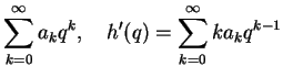
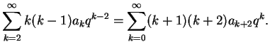
We try to solve this by a power series
We insert these series into (4.12),
![$\displaystyle \sum_{k=0}^{\infty}\left[
(k+1)(k+2)a_{k+2} -2k a_k +(2\varepsilon -1)a_k
\right]q^k=0.$](img1044.png) |
|
|
(238) |
The left side of the equation must be zero for any value of  which can only be true if
all the coefficients in
which can only be true if
all the coefficients in ![$ [...]$](img1046.png) vanish. The powers
vanish. The powers  form an infinite basis
 ;
if any function expanded in this basis is zero, all expansion coefficients must be zero. From
;
if any function expanded in this basis is zero, all expansion coefficients must be zero. From
![$ [...]=0$](img1049.png) in (4.14), we therefore have
in (4.14), we therefore have
 |
|
|
(239) |
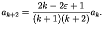
This is a recursion relation for the coefficients  .
For large
.
For large
 , one has
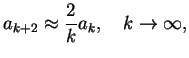 |
|
|
(240) |
unless the become zero above some  .
The infinite power series becomes asymptotical equal to the exponential function
.
The infinite power series becomes asymptotical equal to the exponential function
 for large : consider
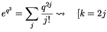 even even![$\displaystyle ]
\frac{a_{k+2}}{a_k}=\frac{(k/2)!}{(k/2+1)!}=\frac{1}{k/2+1}\to \frac{2}{k},\quad k\to \infty.$](img1057.png) |
|
|
(241) |
Now, this is obviously not what we had intended
with our Ansatz, because this would mean that the wave function
 which means
that it is no longer normalizable. The only possibility for a solution that
vanishes as
therefore is obtained by demanding that the
become zero above some
which means
that it is no longer normalizable. The only possibility for a solution that
vanishes as
therefore is obtained by demanding that the
become zero above some  whence becomes a polynomial of finite degree.
For this to be the case, the numerator
in (4.15) has to vanish for some which means
whence becomes a polynomial of finite degree.
For this to be the case, the numerator
in (4.15) has to vanish for some which means
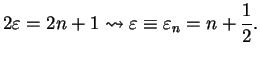 |
|
|
(242) |
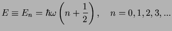
The possible energy values  are therefore
 |
|
|
(243) |
This is the famous quantization of the energy of the harmonic oscillator, which Planck had
postulated to explain the blackbody radiation in 1900!
For each non-negative integer  we obtain one energy eigenvalue and
the corresponding eigenfunction
we obtain one energy eigenvalue and
the corresponding eigenfunction
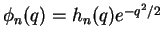 from the finite recursion formula (4.15) for the polynomial
  .
Here, we already use the index to denote the -th solution.
The polynomials
fulfill the differential equation (4.12) with
.
Here, we already use the index to denote the -th solution.
The polynomials
fulfill the differential equation (4.12) with
 , that is
 |
|
|
(244) |
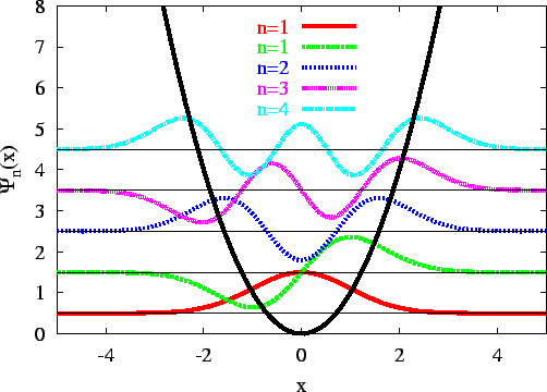
Figure:
Lowest eigenstate wave functions  , Eq.(4.21) of the
one-dimensional harmonic oscillator potential
, Eq.(4.21) of the
one-dimensional harmonic oscillator potential
 (black curve).
Wave functions are in units
(black curve).
Wave functions are in units
 . The curves have an offset for clarity.
 |
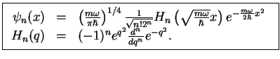
The polynomials that fulfill (4.20)
are called Hermite polynomials  if they are normalized such that the
wavefunctions
if they are normalized such that the
wavefunctions
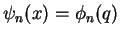 are normalized: the result for the
normalized eigenfunctions with eigenenergy
are normalized: the result for the
normalized eigenfunctions with eigenenergy  , that is the solutions of (4.5),
is
, that is the solutions of (4.5),
is
 |
|
|
(245) |
We do not prove the explicit form of the Hermite polynomials here; in the next section we will
learn an alternative method to calculate the and the anyway.
Here, we calculate  for the first , using (4.21) (denote by
  here)
here)
The lowest eigenfuncions are shown in Fig. (4.1).
Next: The Harmonic Oscillator II
Up: The Harmonic Oscillator I
Previous: Model
Contents
Tobias Brandes
2004-02-04