We have already seen how confinement of particles leads to discrete energies ![]() and wave functions
localized to certain regions of space. Furthermore, we have learned that
the coupling of two separated quantum systems (like the potential wells in section 2.6)
leads to the splitting of energy levels. The tunnel effect couples the left and the right
well and leads to new states that are superpositions, cf. (2.89),
and wave functions
localized to certain regions of space. Furthermore, we have learned that
the coupling of two separated quantum systems (like the potential wells in section 2.6)
leads to the splitting of energy levels. The tunnel effect couples the left and the right
well and leads to new states that are superpositions, cf. (2.89),
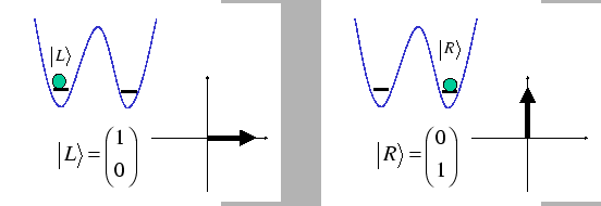
We consider again a system were a particle is moving in a potential that has the form of a double well
like the one in section 2.6. We are interested in the case where
the barrier between the two wells is very high. Let us
concentrate on the wave functions with the lowest energies. We know already that
we can express them approximately by the linear combinations
![]() of
the two lowest states
of
the two lowest states
![]() and
and
![]() of the left and the right well.
of the left and the right well.
We now perform the 5 steps that establish a simple model of what is going on when the two wells become coupled by the barrier:
STEP 1: starting from two isolated wells,
we completely neglect all states apart from the two ground states
in the two wells,
![]() and
and
![]() . We are only interested
in the `low-energy' sector. If both wells have a small width, we know that
the next eigenvalue of the energy is far above the ground state energy so that all
other states are energetically far away from the two ground states
. We are only interested
in the `low-energy' sector. If both wells have a small width, we know that
the next eigenvalue of the energy is far above the ground state energy so that all
other states are energetically far away from the two ground states
![]() and
and
![]() .
.
STEP 2: we now define these two ground states as the two basis vectors of
a complex two-dimensional Hilbert space
![]() . We try to discuss all
the following quantum mechanical features within this `small' Hilbert space which shall be our
approximation of what `really is going on'.
. We try to discuss all
the following quantum mechanical features within this `small' Hilbert space which shall be our
approximation of what `really is going on'.
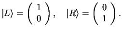
STEP 3: we call the basis vectors
![]() (corresponding to the wave function
(corresponding to the wave function
![]() ) and
) and
![]() (corresponding to the wave function
(corresponding to the wave function
![]() ). We
consider
). We
consider ![]() and
and ![]() just as basis vectors of
just as basis vectors of ![]() . The particular form
of the corresponding wave functions does not interest us. We rather introduce the notation
for basis vectors known from linear algebra, that is
. The particular form
of the corresponding wave functions does not interest us. We rather introduce the notation
for basis vectors known from linear algebra, that is
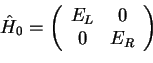
STEP 4: We associate a Hamiltonian ![]() with the two isolated wells:
trivially, the particle is either in the left or in the right well. A measurement
of the energy (the observable belonging to
with the two isolated wells:
trivially, the particle is either in the left or in the right well. A measurement
of the energy (the observable belonging to ![]() ) yields one of the eigenvalues
of
) yields one of the eigenvalues
of ![]() , i.e
, i.e ![]() (the energy of the lowest state left) or
(the energy of the lowest state left) or
![]() (the energy of the lowest state right). In fact, in section 2.6
we always had
(the energy of the lowest state right). In fact, in section 2.6
we always had ![]() but let us be a bit more general here
and allow different ground state energies in both isolated wells.
The Hamiltonian is a two-by-two matrix,
but let us be a bit more general here
and allow different ground state energies in both isolated wells.
The Hamiltonian is a two-by-two matrix,
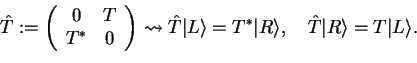
STEP 5 (this is the most abstract step): we now want to incorporate the tunnel effect
when the two wells become coupled by a barrier of finite height. What is the total Hamiltonian
![]() of the system then? A particle initially localized in the left well can now
tunnel into the right well and vice versa. The time-evolution of the wave function is determined
by the total Hamiltonian (remember the time-dependent Schrödinger equation!) which therefore
must contain a term like
of the system then? A particle initially localized in the left well can now
tunnel into the right well and vice versa. The time-evolution of the wave function is determined
by the total Hamiltonian (remember the time-dependent Schrödinger equation!) which therefore
must contain a term like
 |
(188) |
Furthermore, the energies ![]() and
and ![]() are changed: we therefore
write the total Hamiltonian as a sum of three terms,
are changed: we therefore
write the total Hamiltonian as a sum of three terms,
The two-by-two matrix Hamiltonian ![]() , (3.24), is called the Hamiltonian
of the two-level system. It describes the simplest possible quantum mechanical system in terms
of the three parameters
, (3.24), is called the Hamiltonian
of the two-level system. It describes the simplest possible quantum mechanical system in terms
of the three parameters
![]() ,
,
![]() ,
and
,
and ![]() . In spite of its simplicity, this model is the
basis for a lot of phenomena in different fields of physics, such as the dynamics
of emission and absorption of light from atoms, the nuclear magnetic resonance (NMR), the spin
. In spite of its simplicity, this model is the
basis for a lot of phenomena in different fields of physics, such as the dynamics
of emission and absorption of light from atoms, the nuclear magnetic resonance (NMR), the spin ![]() of particles, the physics of semiconductors with two bands (valence and conduction band), and
many others.
of particles, the physics of semiconductors with two bands (valence and conduction band), and
many others.
![\includegraphics[width=0.3\textwidth]{dwell1.eps}](img798.png)
![\includegraphics[width=0.3\textwidth]{dwell2a.eps}](img799.png)
![\includegraphics[width=0.3\textwidth]{dwell2b.eps}](img800.png)