Next: Example: Wave packet
Up: Position and Momentum in
Previous: Position and Momentum in
Contents
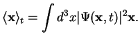
We had seen that the square of the wave function,
 ,
describing a particle in a potential
,
describing a particle in a potential  , is a probability density to find the particle
at
, is a probability density to find the particle
at  at time
  . The result
of a single measurement of can only be predicted to have a certain probability, but
if many measurements of the position under identical conditions
are repeated, the average value (expectation value) of is
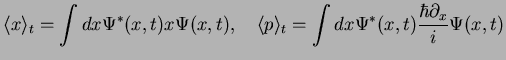
. The result
of a single measurement of can only be predicted to have a certain probability, but
if many measurements of the position under identical conditions
are repeated, the average value (expectation value) of is
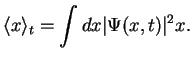 |
|
|
(58) |
We have again adopted a one-dimensional version for simplicity, in three dimensions the expectation value is completely
analogous,
 |
|
|
(59) |
Note that the expectation value is now
a three-dimensional vector which is a function of time . We have indicated the time-dependence
by the notation
 .
.
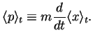
Next, we would like to know the expectation value of the momentum  of the particle.
To determine
of the particle.
To determine  and for a given massive object (like a planet
revolving around the sun) at time is one of the aims of classical mechanics.
In quantum mechanics, we only have the probability density
, but we can calculate
expectation values: We define the expectation value for the momentum
and for a given massive object (like a planet
revolving around the sun) at time is one of the aims of classical mechanics.
In quantum mechanics, we only have the probability density
, but we can calculate
expectation values: We define the expectation value for the momentum  (one-dimensional version) as
 |
|
|
(60) |
This seems plausible because in classical mechanics
 . Later we will see that
an equivalent definition is also possible, using the de Broglie relation
. Later we will see that
an equivalent definition is also possible, using the de Broglie relation  .
We write
.
We write
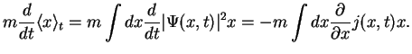
Now, we re-call the definition of the current-density and the continuity equation,
Eq.(1.39),
We therefore find
We compare
 |
|
|
(63) |
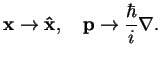
and recognize that
the position  corresponds to the (somewhat trivial) operator `multiplication with '.
On the other hand, the momentum corresponds to the completely non-trivial operator
corresponds to the (somewhat trivial) operator `multiplication with '.
On the other hand, the momentum corresponds to the completely non-trivial operator
 .
A similar calculation leads to
.
A similar calculation leads to
![$\displaystyle \langle x^2 \rangle_t =\int dx \Psi^*({x},t) x^2 \Psi({x},t),\qua...
...t =\int dx \Psi^*({x},t) \left[\frac{\hbar \partial_x}{i}\right]^2 \Psi({x},t).$](img265.png) |
|
|
(64) |
Again, the above can easily be generalized to three dimensions when
 and
and
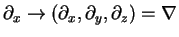 (gradient or Nabla-operator).
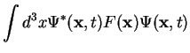
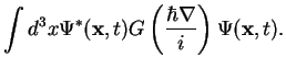
Axiom 2: Expectation values of functions
 of the position or
 of the momentum for a quantum mechanical system described by a wave function
 are calculated
as
are calculated
as
The position corresponds to the operator `multiplication with ', the
momentum to the operator
 , applied to the wave function as in
(1.63),(1.64),(1.65).
, applied to the wave function as in
(1.63),(1.64),(1.65).
This correspondence in particular holds for the total energy, which in classical mechanics
for a conservative system (energy is conserved) is given by a Hamilton function
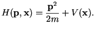 |
|
|
(66) |
The correspondence principle from axiom 2 tells us that this Hamilton function in quantum mechanics
has to be replaced by a Hamilton operator (Hamiltonian) 
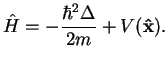 |
|
|
(67) |
Here, we have used the definition of the Laplace operator
 . In Cartesian
coordinates, it is
. In Cartesian
coordinates, it is
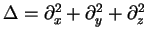 .
The Hamilton operator represents the total energy of the particle with mass
.
The Hamilton operator represents the total energy of the particle with mass  in the potential
 .
We have introduced the hat as a notation for operators, but often the hat is omitted for simplicity.
We make the important observation that is exactly the expression that appears on the right hand
side of
the Schrödinger equation (1.21). This means we can write the Schrödinger equation as
.
We have introduced the hat as a notation for operators, but often the hat is omitted for simplicity.
We make the important observation that is exactly the expression that appears on the right hand
side of
the Schrödinger equation (1.21). This means we can write the Schrödinger equation as
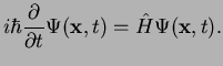 |
|
|
(68) |
This is the most general form of the Schrödinger equation in quantum mechanics. The replacement of
and in quantum mechanics is
Axiom 3: The position and momentum are
operators acting on wave functions,
 |
|
|
(69) |
Next: Example: Wave packet
Up: Position and Momentum in
Previous: Position and Momentum in
Contents
Tobias Brandes
2004-02-04
![$\displaystyle \fbox{$ \begin{array}{rcl} \displaystyle
& &\frac{\partial}{\part...
...si(x,t)
- \Psi(x,t)\frac{\partial}{\partial x}\Psi^*(x,t)\right].
\end{array}$}$](img179.png)
![$\displaystyle {\mbox{\rm [partial integration]}} = m \int dx j(x,t) ={\mbox{\rm [definition of j]}}$](img259.png)
![$\displaystyle -\frac{i\hbar}{2} \int dx
[\Psi^*({x},t)\partial_x \Psi({x},t)-\Psi({x},t)\partial_x \Psi^*({x},t)]
={\mbox{\rm [partial integration]}}$](img260.png)
![$\displaystyle -\frac{i\hbar}{2} \int dx
[\Psi^*({x},t)\partial_x \Psi({x},t)+\partial_x\Psi({x},t) \Psi^*({x},t)]$](img261.png)
![$\displaystyle \int dx [\Psi^*({x},t)\frac{\hbar \partial_x}{i} \Psi({x},t)].$](img262.png)